MGDrivE2: Metapopulation Network Lifecycle Dynamics
Source:vignettes/lifecycle-network.Rmd
lifecycle-network.RmdTable of Contents
- Parameterization
- Initialization of the Petri Net
- Equilibrium Conditions and Hazard Functions
- Simulation of Fully Specified SPN Model
Preface
This vignette describes how to use the facilities provided by MGDrivE2 to run simulations of gene drive dynamics on metapopulation networks; a network of mosquito breeding sites where edges represent the directed per-capita rate of migration between nodes. The movement rates are allowed to be asymmetric and to differ between male and female mosquitoes.
We start by loading the MGDrivE2 package, as well as the MGDrivE package for access to inheritance cubes, ggplot2 for graphical analysis, and Matrix for sparse matrices used in migration. We will use the basic cube to simulate Mendelian inheritance for this example.
# simulation functions
library(MGDrivE2)
#> Loading MGDrivE2: Mosquito Gene Drive Explorer Version 2
# inheritance patterns
library(MGDrivE)
#> Loading MGDrivE: Mosquito Gene Drive Explorer
# plotting
library(ggplot2)
# sparse migration
library(Matrix)

# basic inheritance pattern
cube <- MGDrivE::cubeMendelian()
Parameterization
We specify biological parameter values and equilibrium population
sizes. We will use the same parameter values as in the vignette “MGDrivE2: One Node Lifecycle Dynamics”,
additionally specifying the total simulation time (tmax)
and the timestep to save output (dt).
# entomological parameters
theta <- list(
  qE = 1/4,
  nE = 2,
  qL = 1/3,
  nL = 3,
  qP = 1/6,
  nP = 2,
  muE = 0.05,
  muL = 0.15,
  muP = 0.05,
  muF = 0.09,
  muM = 0.09,
  beta = 16,
  nu = 1/(4/24)
)

# simulation parameters
tmax <- 125
dt <- 1
Initialization of the Petri Net
In order to setup the places and transition of a metapopulation
model, we need to provide data describing the edges between nodes so
that the network can be constructed. First, we make a very simple 2 node
network. We will make a binary matrix adj that indices
whether or not 2 nodes are connected by an edge; the absence of an edge
means that movement between those two nodes is not possible. We use the
sparseMatrix class from the Matrix package
because, for larger network topologies, the sparse matrix representation
may have significant benefits. It should be specified with the diagonal
empty, because we do not consider “migration” to your current
location.
Next, we can setup all of the places in the model, provided the entomological parameters above, the inheritance pattern, and the size of the network.
Then, we create all of the possible transitions between states, given the places in the model and the network adjacency matrix.
Finally, as not all transitions apply to all “places”, we create a
summary of possible transitions to and from each “place”. This is
handled by the spn_S() function.
# adjacency matrix
#  specify where individuals can migrate
adj <- Matrix::sparseMatrix(i = c(1,2),j = c(2,1))
n <- nrow(adj)

# Places and transitions
SPN_P <- spn_P_lifecycle_network(num_nodes = n, params = theta,cube = cube)
SPN_T <- spn_T_lifecycle_network(spn_P = SPN_P, params = theta,cube = cube,m_move = adj)

# Stoichiometry matrix
S <- spn_S(spn_P = SPN_P, spn_T = SPN_T)
Equilibrium Conditions and Hazard Functions
Now that the structural properties of the SPN model have been set up,
we will calculate equilibrium population sizes, M0. We will
use the same parameter values as in the vignette “MGDrivE2 One Node Lifecycle Dynamics”.
Note that when setting M0 we only set the wild-type
populations; the equilibrium calculations assume a wildtype population
in equilibrium at
.
# now that we have a network size, set adult females in each node
NF <- rep(x = 500, times = n)

# calculate equilibrium and setup initial conditions
#  outputs required parameters in the named list "params"
#  outputs intial equilibrium for adv users, "init
#  outputs properly filled initial markings, "M0"
initialCons <- equilibrium_lifeycle(params = theta, NF = NF, phi = 0.5,
                                    log_dd = TRUE, spn_P = SPN_P, cube = cube)
Before making the hazard functions and finishing the SPN, we need to
calculate movement rates (because in MGDrivE2, the
movement matrix is a matrix of per-capita movement rates rather
than probabilities; matrix exponentiation would give corresponding
probabilities over a time interval). We use the helper function
calc_move_rate(), which calculates total per-capita rate of
movement out of a node based on mortality rate and the probability to
leave that node before dying.
The vector move_rates is the total rate at which a
mosquito leaves a node, and the sparseMatrix object
move_probs is the conditional probability of where it goes,
given it has chosen to leave; we make movement uniform (although it
won’t matter in the 2-node case, leaving node 1 means they will always
go to node 2). Finally, we attach these objects to the list of
parameters initialCons$params.
# calculate movement rates and movement probabilities
gam <- calc_move_rate(mu = theta$muF, P = 0.05)

move_rates <- rep(x = gam, times = n)
move_probs <- Matrix::sparseMatrix(i = {}, j = {},x = 0L,dims = dim(adj))

# uniform movement probabilities
rowprobs <- 1/rowSums(adj)
for(i in 1:nrow(move_probs)){
  cols <- Matrix::which(adj[i,])
  move_probs[i,cols] <- rep(rowprobs[i],length(cols))
}

# put rates and probs into the parameter list
initialCons$params$mosquito_move_rates <- move_rates
initialCons$params$mosquito_move_probs <- move_probs
Now that all the necessary parameters have been added to the named
list initialCons$params, we can generate the hazard
functions. By specifying log_dd = TRUE, we use logistic
density dependence for these simulations.
# approximate hazards for continous approximation
approx_hazards <- spn_hazards(spn_P = SPN_P, spn_T = SPN_T, cube = cube,
                              params = initialCons$params, type = "life",
                              log_dd = TRUE, exact = FALSE, tol = 1e-6,
                              verbose = FALSE)

# exact hazards for integer-valued state space
exact_hazards <- spn_hazards(spn_P = SPN_P, spn_T = SPN_T, cube = cube,
                             params = initialCons$params, type = "life",
                             log_dd = TRUE, exact = TRUE, tol = NaN,
                             verbose = FALSE)
Simulation of Fully Specified SPN Model
Now that the structural elements of the Petri Net have been built,
and we have a vector of hazard functions, we can simulate dynamics on
the network. First, we will make a data.frame to hold
information about the releases; We will release 50 adult females with
homozygous recessive alleles 5 times, every 10 days, starting at day 20,
and only in node 1. It is critically important that the event
names match a place name in the simulation. The simulation
function checks this and will throw an error if the event name does not
exist as a place in the simulation. This format is used in
MGDrivE2 for consistency with solvers in
deSolve.
# releases
r_times <- seq(from = 20, length.out = 5, by = 10)
r_size <- 50
events <- data.frame("var" = paste0("F_", cube$releaseType, "_", cube$wildType, "_1"),
                     "time" = r_times,
                     "value" = r_size,
                     "method" = "add",
                     stringsAsFactors = FALSE)
Deterministic: ODE Solutions
First we run a mean-field approximation of the stochastic model.
Internally, MGDrivE2 uses the high quality numerical
solvers in deSolve to integrate a mean-field approximation
to the stochastic model. We also plot the adult dynamics for both nodes
so we can see how the releases spread through the network.
# run deterministic simulation
ODE_out <- sim_trajectory_R(x0 = initialCons$M0, tmax = tmax, dt = dt, S = S,
                            hazards = approx_hazards, sampler = "ode", method = "lsoda",
                            events = events, verbose = FALSE)

# summarize females/males by genotype
ODE_female <- summarize_females(out = ODE_out$state, spn_P = SPN_P)
ODE_male <- summarize_males(out = ODE_out$state)

# add sex for plotting
ODE_female$sex <- "Female"
ODE_male$sex <- "Male"

# plot
ggplot(data = rbind(ODE_female, ODE_male)) +
  geom_line(aes(x = time, y = value, color = genotype)) +
  facet_grid(node ~ sex, scales = "fixed") +
  theme_bw() +
  ggtitle("SPN: ODE solution")
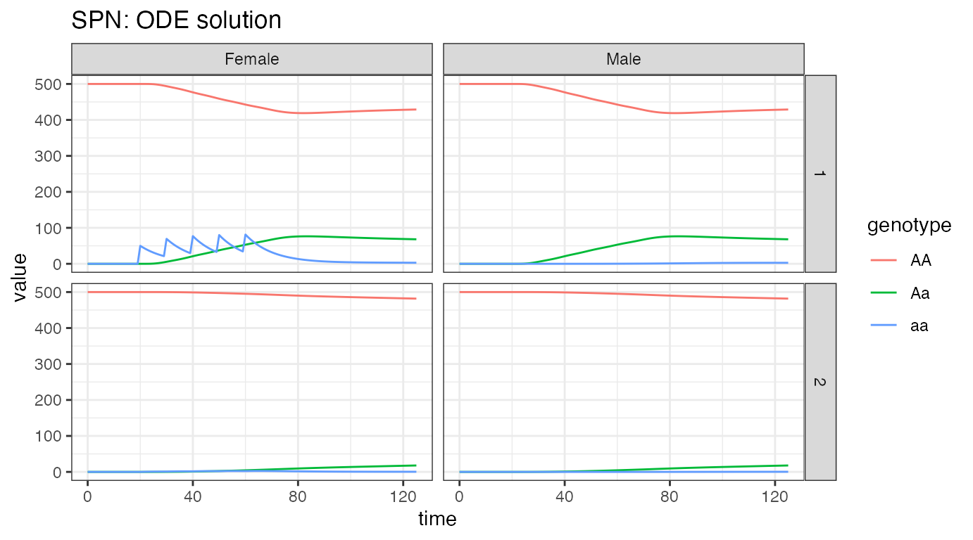
From the plots, we see the initial equilibria in both patches is 500
individuals, the same for each sex, as specified above. We see the
releases in node 1 females, and how they quickly spread into the
population, becoming evenly spread between females and males. In node 2,
we see a much slower introgression of a alleles, all as
heterozygous Aa, due to the very low migration rate between
nodes. If run long enough, we would eventually see all genotype
frequencies reach their equilibrium values in both nodes.
Stochastic: Tau-leaping Solutions
As a further example, we run a single stochastic realization of the same network, using a tau-leaping method with .
# delta t
dt_stoch <- 0.1

# tau leaping simulation
PTS_out <- sim_trajectory_R(x0 = initialCons$M0, tmax = tmax, dt = dt,
                            dt_stoch = dt_stoch, S = S, hazards = exact_hazards,
                            sampler = "tau", events = events, verbose = FALSE)

# summarize females/males by genotype
PTS_female <- summarize_females(out = PTS_out$state, spn_P = SPN_P)
PTS_male <- summarize_males(out = PTS_out$state)

# add sex for plotting
PTS_female$sex <- "Female"
PTS_male$sex <- "Male"

# plot
ggplot(data = rbind(PTS_female, PTS_male)) +
  geom_line(aes(x = time, y = value, color = genotype)) +
  facet_grid(node ~ sex, scales = "fixed") +
  theme_bw() +
  ggtitle("SPN: Tau-leaping Approximation")
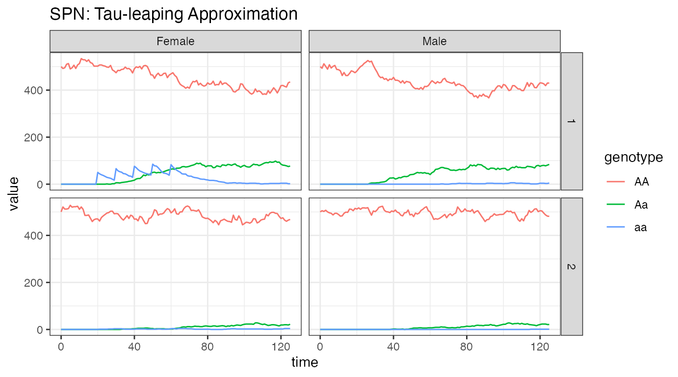
We see a heuristically similar figure as above. This is only 1 stochastic realization, but it closely follows the dynamics from the ODE solver, indicating that a time-step of 0.1 provides and accurate simulation at this level.