MGDrivE2: One Node Epidemiological Dynamics - Decoupled SIS Sampling • MGDrivE2

Parameterization
Initialization of the Petri Net
Equilibrium Conditions and Hazard Functions
Simulation of Fully Specified SPN Model
1. Deterministic: ODE Solutions
2. Stochastic: CLE Solutions
References

Preface

In this vignette, we show a proof-of-concept of a new sampling framework in which the mosquito dynamics are decoupled from the human dynamics. The two systems pass relevant information to each other at time step for the duration of the simulation. The motivation for decoupling the human and mosquito dynamics is to be able to incorporate more complex models of disease transmission into MGDrivE-2’s sampling framework. While this vignette shows a simple SIS model, the eventual goal is to incorporate the Imperial College model of malaria transmission (https://www.researchsquare.com/article/rs-72317/v1) to model the epidemiological effects of gene drive organisms. This model, alongside other complex models, are not directly compatible with MGDrivE-2’s stochastic Petri net (SPN) architecture due to continuous-state immunity functions and non-Markovian delays, and therefore are separated into their own module. Future vignettes will showcase the decoupled functionality with the Imperial model, but here we showcase the functionality with an SIS model.

In this way, we can still leverage the entomological simulations furnished by MGDrivE-2 and apply the relevant parameters to the epidemiological module. This framework also allows for other models of disease transmission to be swapped in when needed. Here, only the mosquito component functions as an SPN, whereas the human component is formulated using ODEs. For a more complete overview of the decoupled sampling framework, see: https://www.overleaf.com/read/hhwbxpqnhzfv

We start by loading the MGDrivE2 package, as well as the MGDrivE package for access to inheritance cubes and ggplot2 for graphical analysis. We will use the basic cube to simulate Mendelian inheritance for this example.

# simulation functions
library(MGDrivE2)
#> Loading MGDrivE2: Mosquito Gene Drive Explorer Version 2
# inheritance patterns
library(MGDrivE)
#> Loading MGDrivE: Mosquito Gene Drive Explorer
# plotting
library(ggplot2)

# basic inheritance pattern
cube <- MGDrivE::cubeMendelian()

Parameterization

Several parameters are necessary to setup the structural properties of the Petri Net, as well as calculate the population distribution at equilibrium, setup initial conditions, and calculate hazards. Again, we specify all entomological parameters as for the mosquito-only simulation (see “MGDrivE2: One Node Lifecycle Dynamics”) as well as additional parameters for the SEI mosquito dynamics. Like the aquatic stages, $\frac{1}{q_{\mathit{EIP}}}$ will give the mean dwell time for incubating mosquitoes, and variance by $\frac{1}{n_{\mathit{EIP}} \cdot q_{\mathit{EIP}}^{2}}$ . The model requires muH, mortality rate in humans, because equilibrium dynamics are simulated (that is, human populations follow an “open cohort” with equal birth and death rates). A table of (case-sensitive) epidemiological parameters the user needs to specify is given below. Note that all parameters must be specified as a rate per day. For a detailed discussion of these parameters in the context of malaria models, see Smith and McKenzie (2004).

Parameter	Description
`NH`	total human population size
`X`	equilibrium prevalence of disease in humans
`f`	mosquito feeding rate
`Q`	proportion of blood meals taken on humans (human blood index in field literature)
`b`	mosquito to human transmission efficiency
`c`	human to mosquito transmission efficiency
`r`	rate of recovery in humans
`muH`	mortality rate in humans
`qEIP`	inverse of mean duration of EIP
`nEIP`	shape parameter of Erlang-distributed EIP

Please note that f and Q must be specified; this is because future versions of MGDrivE2 will include additional vector control methods such as IRS (indoor residual spraying) and ITN (insecticide treated nets). In the presence of ITNs/IRS f will vary independently as a function of time depending on intervention coverage.

Additionally, we specify a total simulation length of 300 days, with output stored daily.

# entomological and epidemiological parameters
theta <- list(
  # lifecycle parameters
  qE = 1/4,
  nE = 2,
  qL = 1/3,
  nL = 3,
  qP = 1/6,
  nP = 2,
  muE = 0.05,
  muL = 0.15,
  muP = 0.05,
  muF = 0.09,
  muM = 0.09,
  beta = 16,
  nu = 1/(4/24),
  # epidemiological parameters
  NH = 1000,
  X = 0.25,
  f = 1/3,
  Q = 0.9,
  b = 0.55,
  c = 0.15,
  r = 1/200,
  muH = 1/(62*365),
  qEIP = 1/11,
  nEIP = 6
)
theta$a <- theta$f*theta$Q

# simulation parameters
tmax <- 250
dt <- 1

We also need to augment the cube with genotype specific transmission efficiencies; this allows simulations of gene drive systems that confer pathogen-refractory characteristics to mosquitoes depending on genotype. The specific parameters we want to attach to the cube are b and c, the mosquito to human and human to mosquito transmission efficiencies. We assume that transmission from human to mosquito is not impacted in modified mosquitoes, but mosquito to human transmission is significantly reduced in modified mosquitoes. For detailed descriptions of these parameters for modeling malaria transmission, see Smith & McKenzie (2004) for extensive discussion. These genotype-specific transmission efficiencies are used in the human ODE model to determine the rates of movement between susceptible and infected compartments.

# augment the cube with RM transmission parameters
cube$c <- setNames(object = rep(x = theta$c, times = cube$genotypesN), nm = cube$genotypesID)
cube$b <- c("AA" = theta$b, "Aa" = 0.35, "aa" = 0)

Initialization of the Petri Net

The SEI disease transmission model sits “on top” of the existing MGDrivE2 structure, using the default aquatic and male “places”, but expanding adult female “places” to follow an Erlang-distributed pathogen incubation period (called the extrinsic incubation period, EIP). Information on how to choose the proper EIP distribution can be found in the help file for ?makeQ_SEI().

The transitions between states is also expanded, providing transitions for females to progress in infection status, adding human dynamics, and allowing interaction between mosquito and human states. All of these additions are handled internally by spn_T_epiSIS_node(). Since only the mosquito portion is stochastic, the SPN will only include the mosquito states. Human states will be handled by the sampling algorithm in the form of a deterministic ODE.

# Places and transitions
# note decoupled sampling is only supported currently for one node.
SPN_P <- spn_P_epi_decoupled_node(params = theta, cube = cube)
SPN_T <- spn_T_epi_decoupled_node(spn_P = SPN_P, params = theta, cube = cube)

# Stoichiometry matrix
S <- spn_S(spn_P = SPN_P, spn_T = SPN_T)

Equilibrium Conditions and Hazard Functions

Now that we have set up the structural properties of the Petri Net, we need to calculate the population distribution at equilibrium and define the initial conditions for the simulation.

The function equilibrium_SEI_SIS() calculates the equilibrium distribution of female mosquitoes across SEI stages, based on human populations and force-of-infection, then calculates all other equilibria. We set the logistic form for larval density-dependence in these examples by specify log_dd = TRUE.

# SEI mosquitoes and SIS humans equilibrium
#  outputs required parameters in the named list "params"
#  outputs initial equilibrium for adv users, "init
#  outputs properly filled initial markings, "M0"
initialCons <- equilibrium_SEI_decoupled_mosy(params = theta, phi = 0.5, log_dd = TRUE,
                                   spn_P = SPN_P, cube = cube)

# augment with human equilibrium states
initialCons$H <- equilibrium_SEI_decoupled_human(params = theta)

With the equilibrium conditions calculated (see ?equilibrium_SEI_SIS()), and the list of possible transitions provided by spn_T_epiSIS_node(), we can now calculate the rates of those transitions between states.

# approximate hazards for continuous approximation
approx_hazards <- spn_hazards_decoupled(spn_P = SPN_P, spn_T = SPN_T, cube = cube,
                              params = initialCons$params, type = "SIS",
                              log_dd = TRUE, exact = FALSE, tol = 1e-8,
                              verbose = FALSE)

Simulation of Fully Specified SPN Model

Similar to previous simulations, we will release 50 adult females with homozygous recessive alleles 5 times, every 10 days, but starting at day 20. Remember, it is critically important that the event names match a place name in the simulation. The simulation function checks this and will throw an error if the event name does not exist as a place in the simulation. This format is used in MGDrivE2 for consistency with solvers in deSolve.

# releases
r_times <- seq(from = 20, length.out = 5, by = 10)
r_size <- 50
events <- data.frame("var" = paste0("F_", cube$releaseType, "_", cube$wildType, "_S"),
                     "time" = r_times,
                     "value" = r_size,
                     "method" = "add",
                     stringsAsFactors = FALSE)

Stochastic: Tau Leaping Solutions

As a further example, we run a single stochastic realization of the same simulation, using the tau-decoupled sampler with $\Delta t = 1$ , approximating 10 jumps per day. This means that we use a tau-leaping sampler in the mosquito states’ SPN, and ODE integration the human model. As the adult male mosquitoes do not contribute to infection dynamics, we will only view the adult female mosquito and human dynamics here.

# delta t - one day
dt_stoch <- 0.1

# run tau-leaping simulation
tau_out <- sim_trajectory_R_decoupled(
  x0 = initialCons$M0,
  h0 = initialCons$H,
  SPN_P = SPN_P,
  theta = theta,
  tmax = tmax,
  inf_labels = SPN_T$inf_labels,
  dt = dt,
  dt_stoch = dt_stoch,
  S = S,
  hazards = approx_hazards,
  sampler = "tau-decoupled",
  events = events,
  verbose = FALSE,
  human_ode = "SIS",
  cube = cube
)

# summarize females/humans by genotype
tau_female <- summarize_females_epi(out = tau_out$state, spn_P = SPN_P)
tau_humans <- summarize_humans_epiSIS(out = tau_out$state)

# plot
ggplot(data = rbind(tau_female, tau_humans) ) +
  geom_line(aes(x = time, y = value, color = inf)) +
  facet_wrap(~ genotype, scales = "free_y") +
  theme_bw() +
  ggtitle("SPN: Tau Decoupled Solution")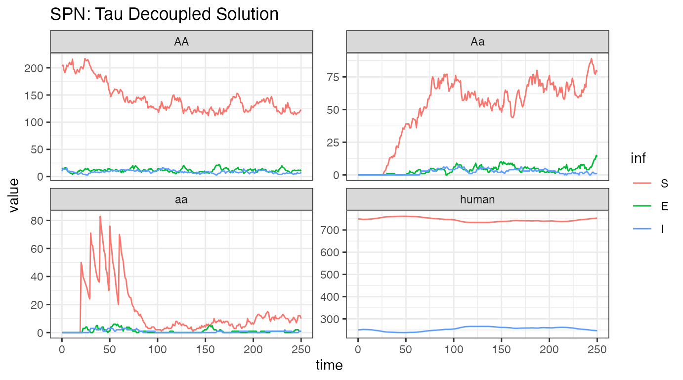

Analyzing one stochastic realization of this system, we see some similarities and some striking differences. The releases are clearly visible, lower left-hand plot, and we see that the initial dynamics are similar to the ODE dynamics. However, it is quickly apparent that the releases are not reducing transmission adequately, that in fact, disease incidence is increasing rapidly in human and female mosquitoes. There are two main possibilities for this: first, that the stochastic simulation just happens to drift like this, a visual reminder that there can be significant differences when the well-mixed, mean-field assumptions are relaxed, or that the step size ( $\Delta t$ ) is too large, and the stochastic simulation is a poor approximation of the ODE solution. Further tests, with $\Delta t = 0.05$ and $\Delta t = 0.15$ , returned similar results, indicating that this is an accurate approximation but still highlighting the importance of testing several values of $\Delta t$ for consistency.

References

Smith, D. L., & McKenzie, F. E. (2004). Statics and dynamics of malaria infection in Anopheles mosquitoes. Malaria journal, 3(1), 13.

MGDrivE2: One Node Epidemiological Dynamics - Decoupled SIS Sampling